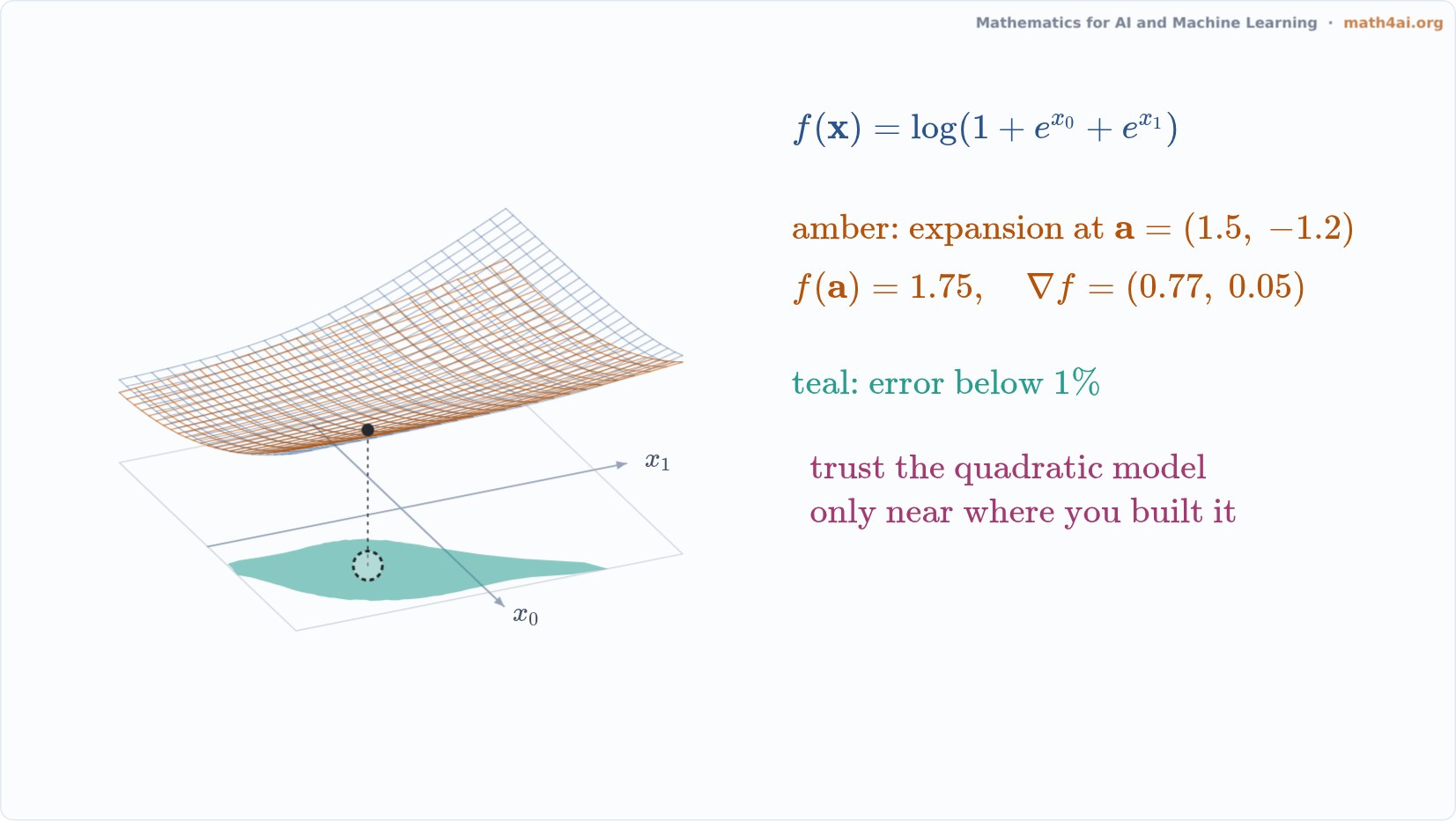
Second-Order Taylor: Where the Quadratic Model Can Be Trusted
A narrated live film: a function, its second-order Taylor bowl, and the region where the bowl is accurate, all moving with the expansion point in 3D.
Narration
Here is the surface of f, the log of one plus e to the x zero plus e to the x one, and its second order Taylor expansion at the origin: the amber bowl. The value log three, the gradient one third, one third, and the Hessian build that bowl.
Near the origin, the two surfaces are almost the same. The teal region on the floor marks where the error is below one percent. Farther away, the bowl curves up, while f keeps growing almost linearly.
The rest of the narration is in the book's Companion.
More from Chapter 11
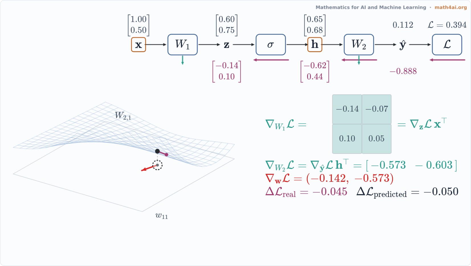 Interactive1:54Backpropagation, One VJP per LayerChapter 11
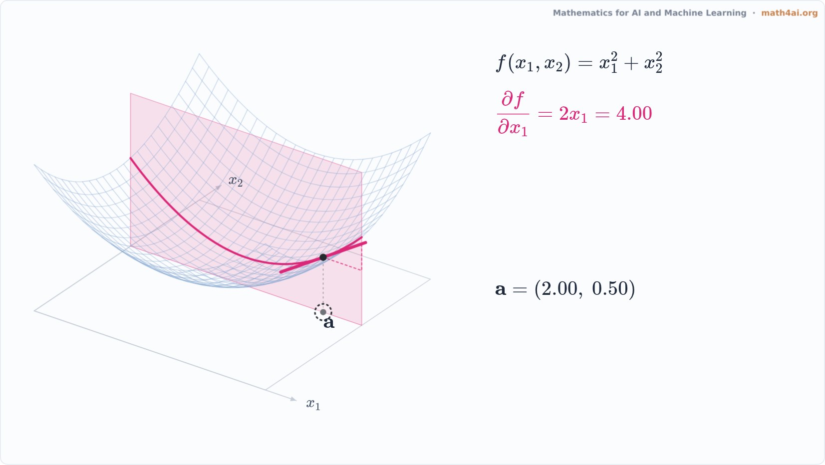 Preview1:27Partial Derivatives Are Two SlicesChapter 11
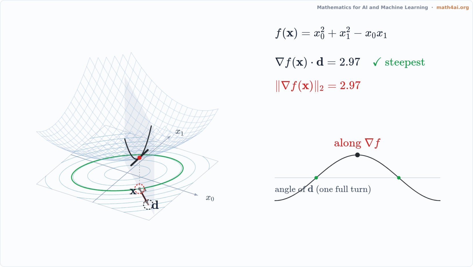 Preview1:34The Gradient Is the Steepest DirectionChapter 11
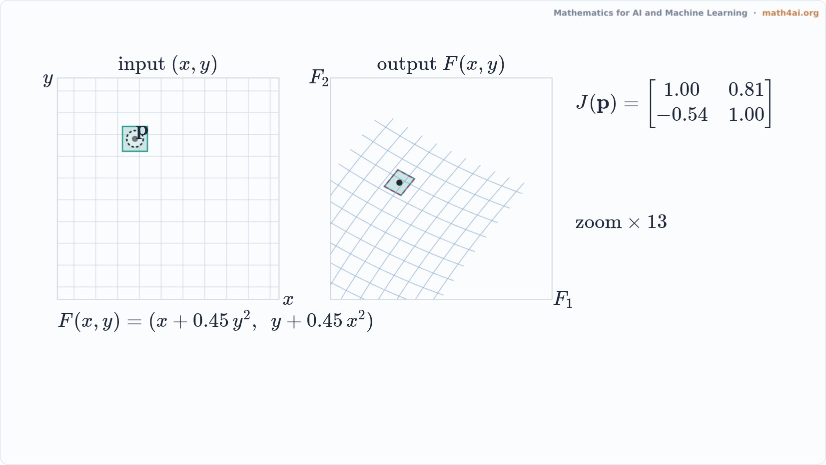 Preview1:42Jacobian Matrix: Linearizing a MapChapter 11
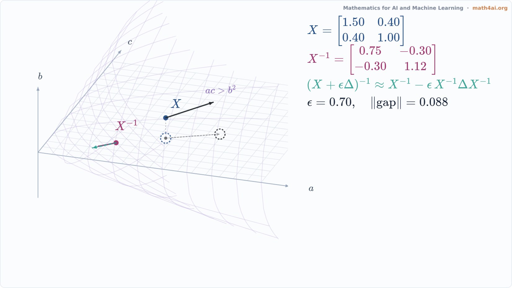 Preview1:43The Derivative of the Matrix InverseChapter 11
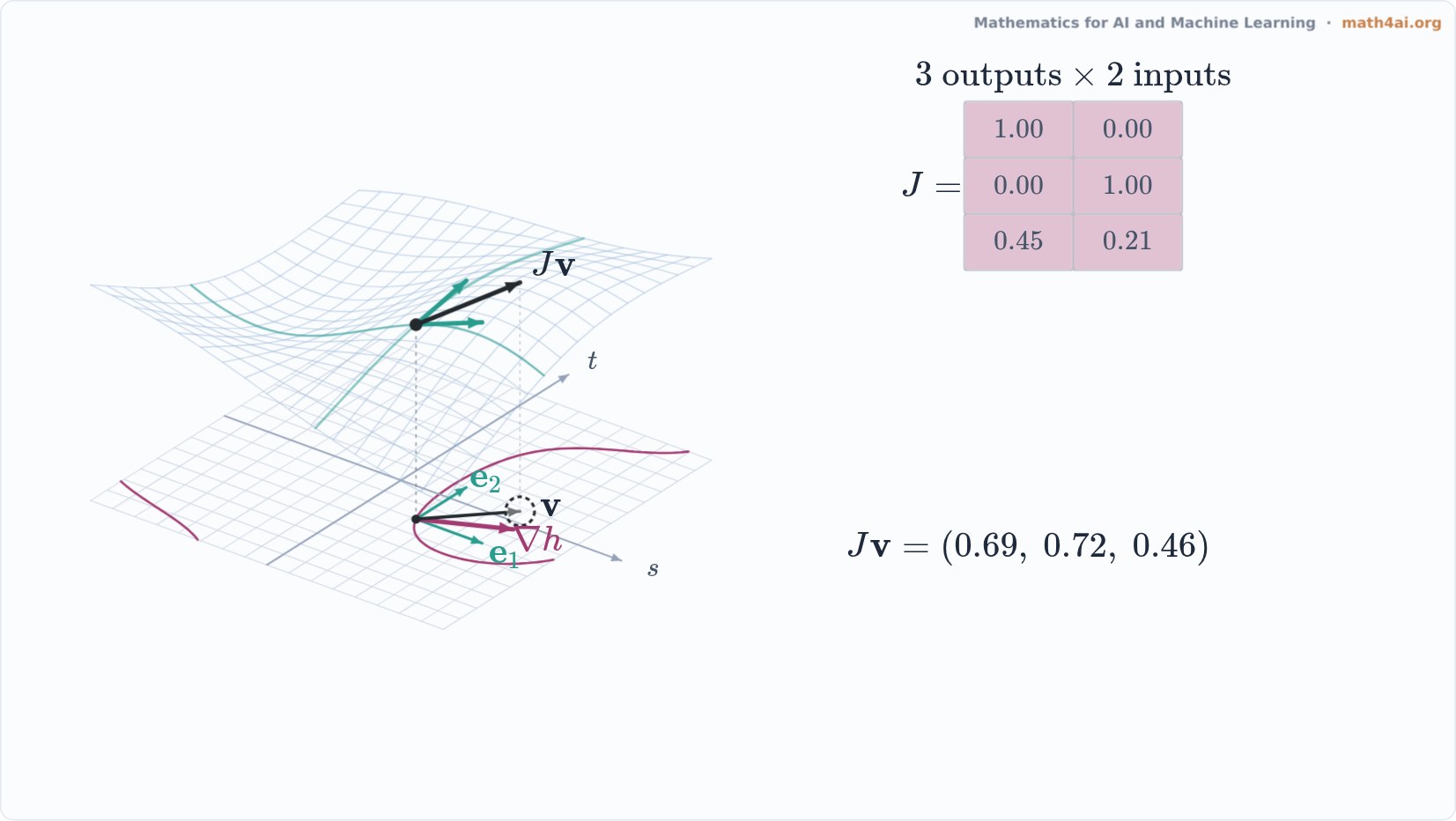 Preview1:54Forward or Reverse: Filling the JacobianChapter 11
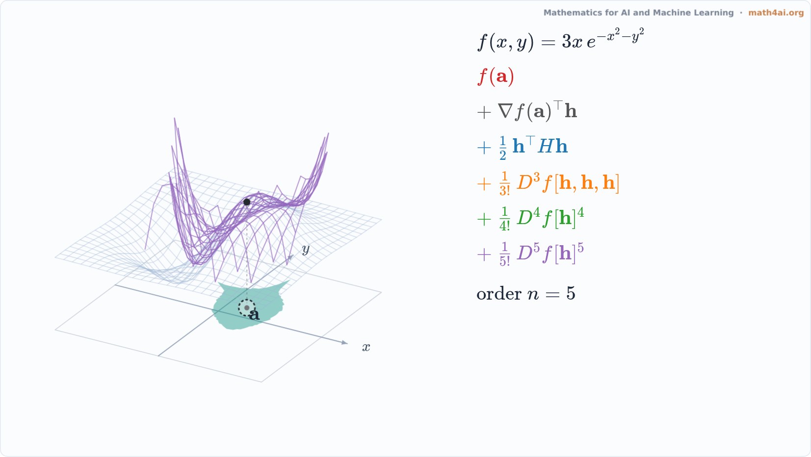 Preview1:32Taylor Expansion, One Term at a TimeChapter 11
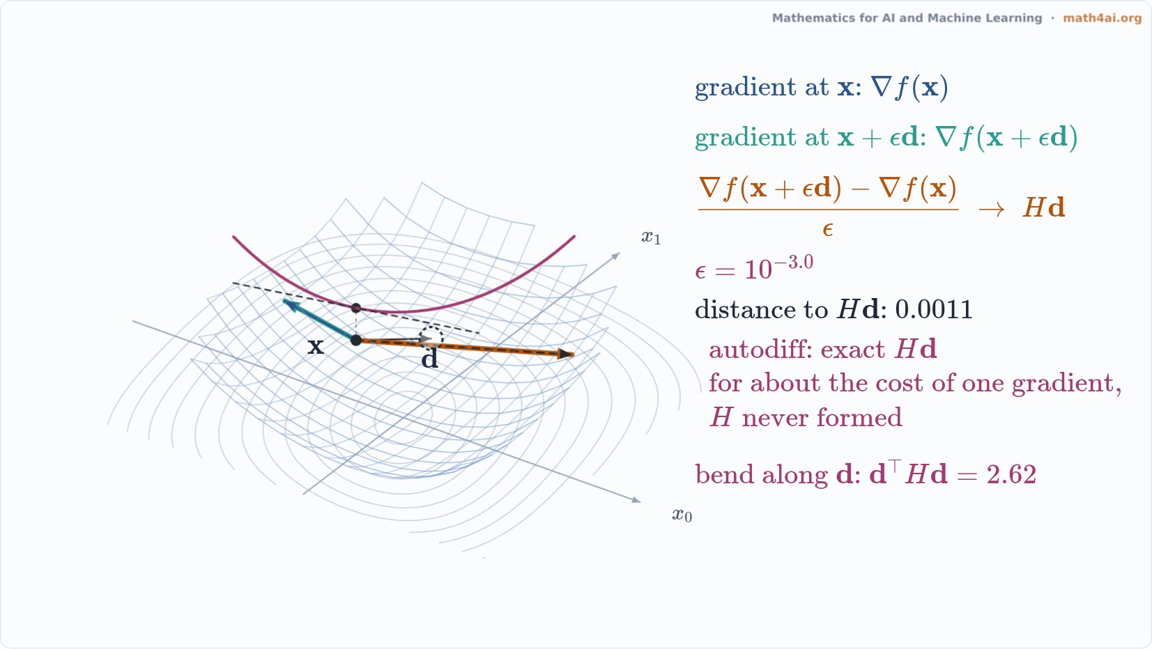 Preview1:38A Hessian-Vector Product from Two GradientsChapter 11
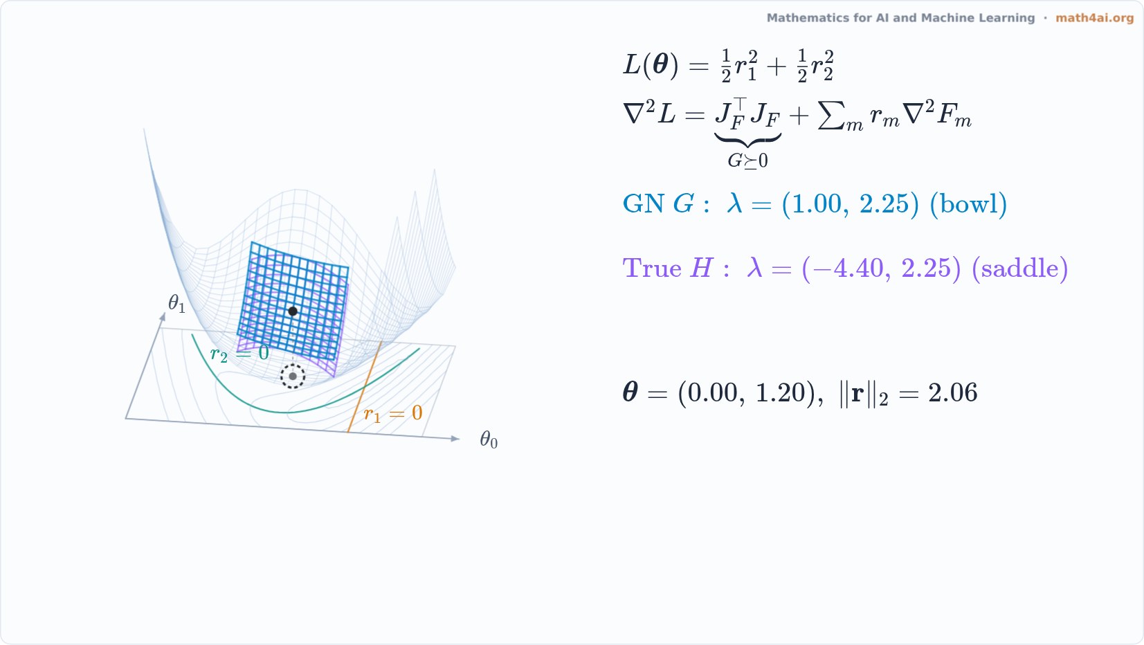 Preview1:34The Gauss–Newton MatrixChapter 11
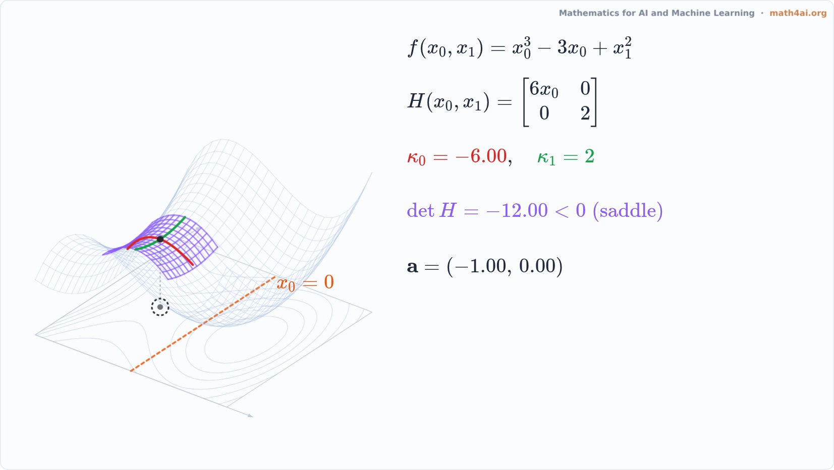 Preview1:44Hessian Matrix: Bowls, Saddles and Curvature DirectionsChapter 11
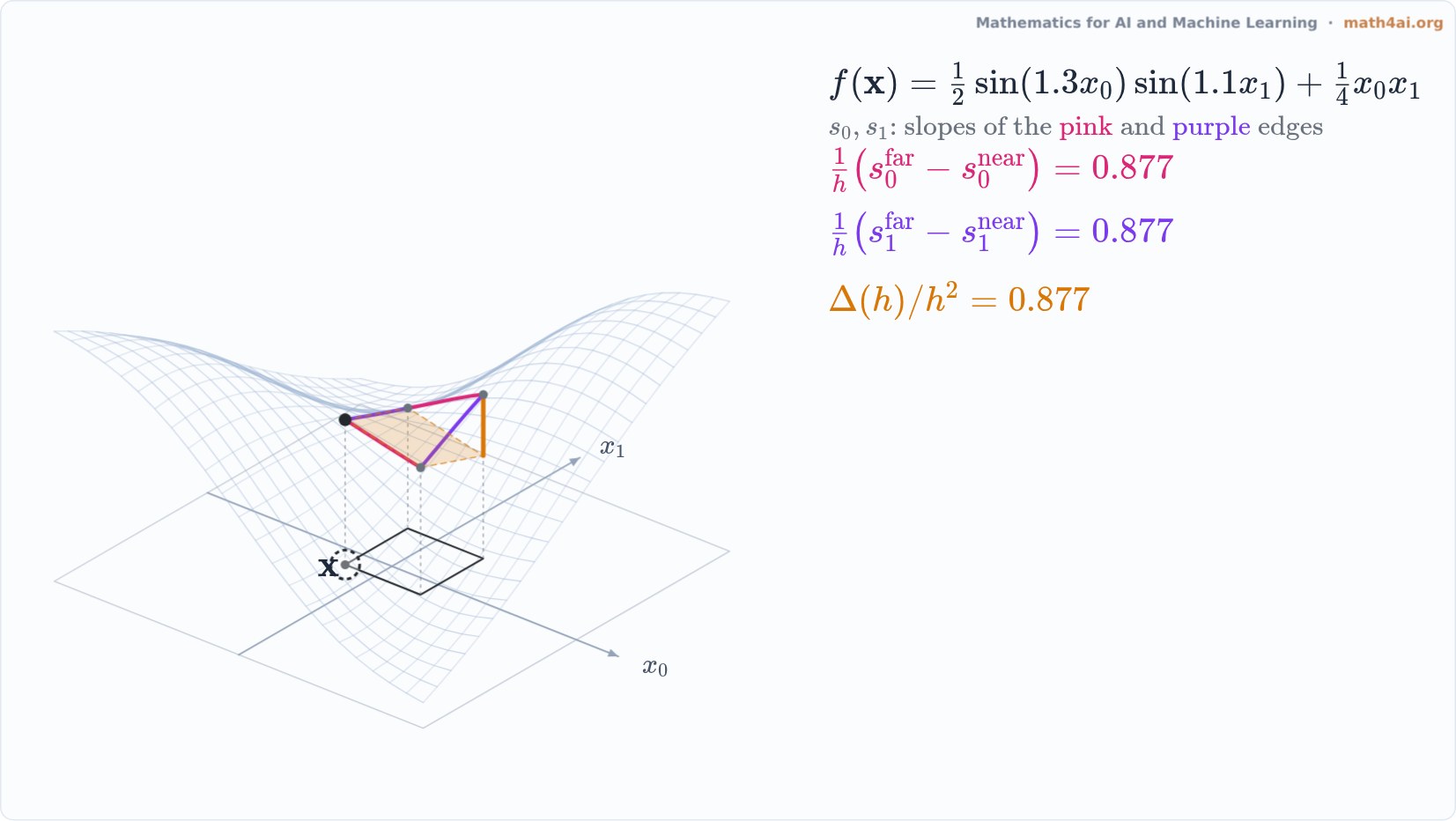 Preview1:37Why the Hessian Is SymmetricChapter 11
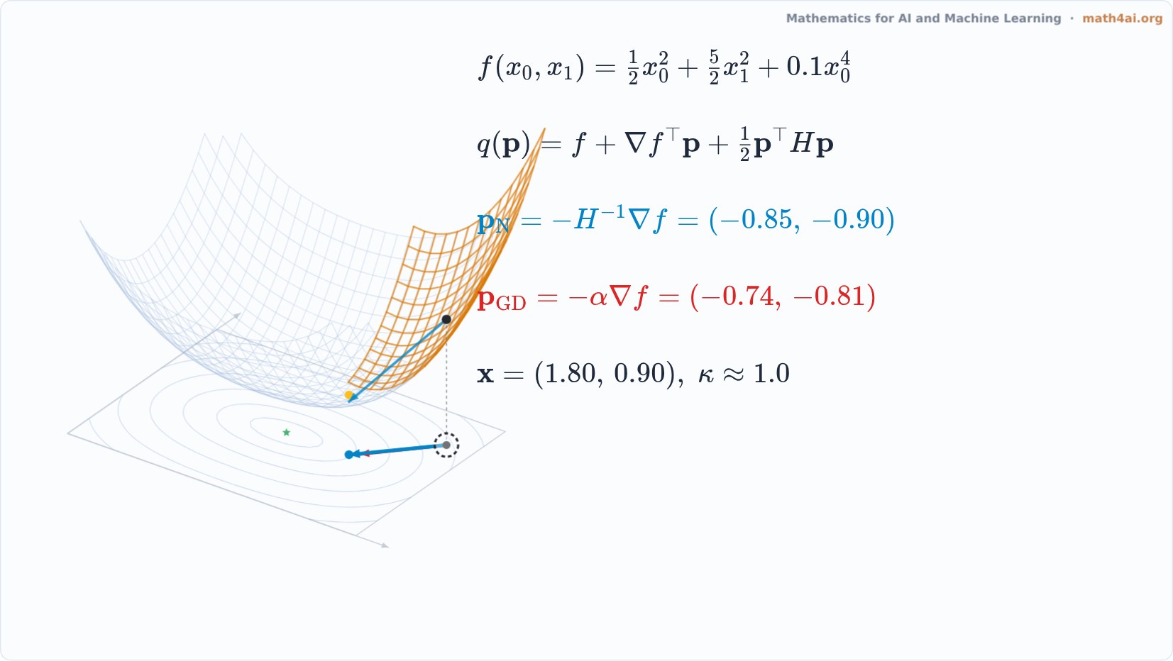 Preview1:26The Newton Step: Jumping to the Taylor Bowl's BottomChapter 11
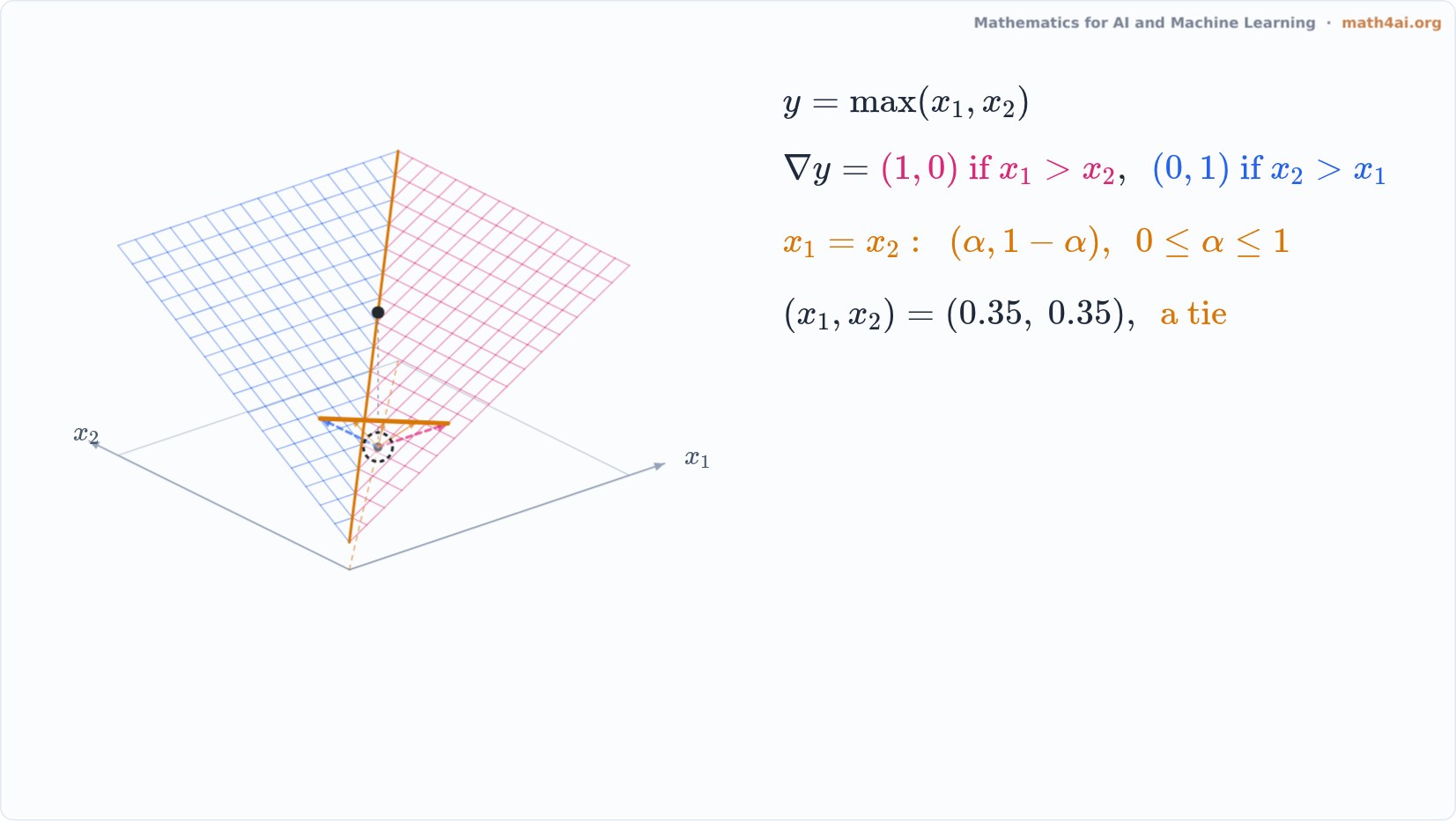 Preview2:36Corners, Maxima and Steps in the Chain RuleChapter 11
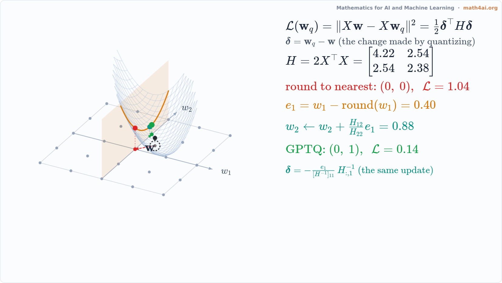 Preview1:59GPTQ: Rounding with the HessianChapter 11
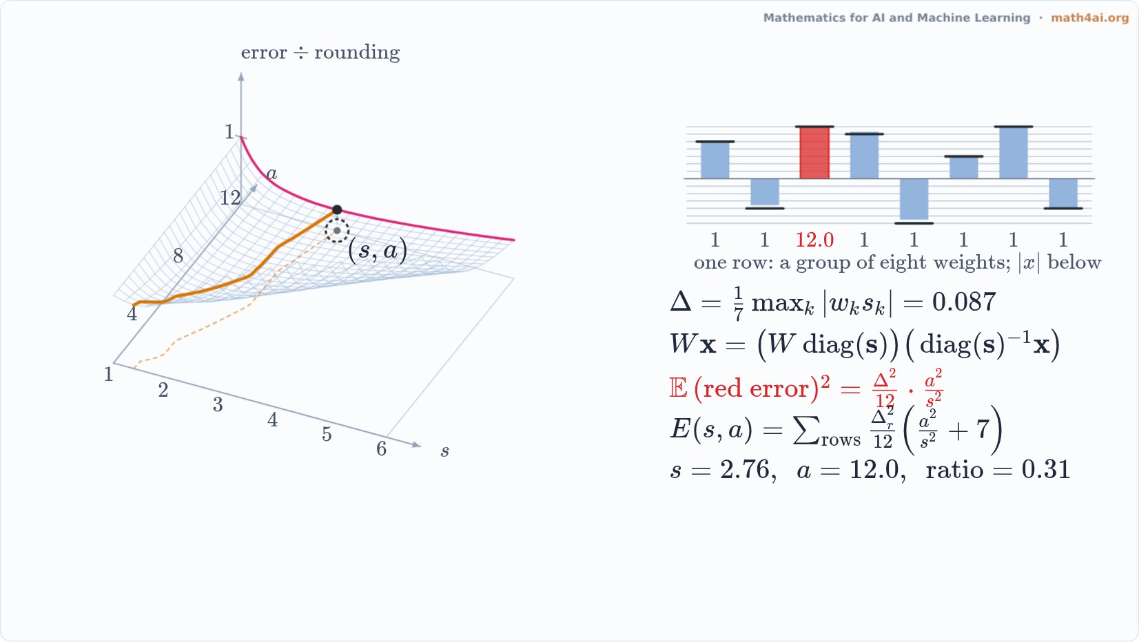 Preview2:12AWQ: Activation-Aware Weight QuantizationChapter 11
 Preview1:41The Implicit Function TheoremChapter 11